Deep Neural Network for MNIST Handwriting Recognition
I finally found some time to enhance my neural network to support deep learning. The network now masters a variable number of layers and is capable of running convolutional layers. The architecture is generic, light weight (very small memory footprint) and super fast. :-)
![]()
In a previous blog post I wrote about a simple 3-Layer neural network for MNIST handwriting recognition that I built. Its architecture -- a 3-layer structure with exactly 1 hidden layer -- was fix. And it only supported normal fully connected layers.
To achieve better results in image recognition tasks deeper networks are needed. And, ideally, they need to be capable of running convolutional layers. Hence, I set out to add these features, on my continous journey into the world of machine learning. :)
Convolutional Networks
Convolutional layers are a different beast than normal fully connected layers. Instead of each node in a layer connecting to all nodes in the previous layer, it connects to only some of them. The selection of which nodes it connects to is defined by a quadratic filter that moves over the previous layer. The geolocation of each node, i.e. the horizontal and vertical proximity to its neighbors, is thereby taken into account which is crucial for image recognition.
The second major difference of convolutional layers is the fact that weights are shared between nodes. This siginificantly reduces the network's complexity, i.e. the number of weights or parameters that need to be trained, as well as its memory requirements.
This post assumes that you understand the basic functionality of a convolutional network. If you don't I strongly recommend reading Stanford's CS231n Convolutional Neural Networks for Visual Recognition by Andrej Karpathy or, more hardcore, Yann Lecun's LeNet-5 Convolutional Neural Networks first.
So, now let's jump into the code and start with the network's overall design.
Network Architecture
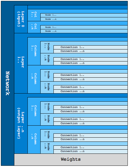
More than anything else did the introduction of convolutional layers influence the design of the network. Previously, my network structure consisted of layers, nodes and weights. Now, I added 2 additional concepts: Columns and Connections.
So in total, the neural network consists of 5 data structures.
The Network
The network structure serves as the overall container for the whole network. It defines the learning rate and information about number and location of all weights in the network. And, most importantly, it includes a variable-sized array of layer structures which contain the network nodes.
1struct Network{
2    ByteSize size;                  // actual byte size of this structure in run-time
3    double learningRate;            // factor by which connection weight changes are applied
4    int weightCount;                // number of weights in the net's weight block
5    Weight *weightsPtr;             // pointer to the start of the network's weights block
6    Weight nullWeight;              // memory slot for a weight pointed to by dead connections
7    int layerCount;                 // number of layers in the network
8    Layer layers[];                 // array of layers (of different sizes)
9};
A Network Layer
The Layer structure contains all the information related to a specific layer in the network, including a pointer to its weights and a variable-sized array of all columns inside this layer.
It's worth mentioning here that in my design, the input layer is counted as one of the layers. Other definitions may vary. Yann LeCun's collection of MNIST results, for example, defines a linear classifier as a 1-layer-NN, and networks with exactly 1 hidden layer as 2-layer-NNs. In my design these count as 2-layer-NN and 3-layer-NN respectively.
1struct Layer{
2    int id;                         // index of this layer in the network
3    ByteSize size;                  // actual byte size of this structure in run-time
4    LayerDefinition *layerDef;      // pointer to the definition of this layer
5    Weight *weightsPtr;             // pointer to the weights of this layer
6    int columnCount;                // number of columns in this layer
7    Column columns[];               // array of columns
8};
The second point worth mentioning here is that I keep the definition of the layer model outside of the Layer structure in a separate LayerDefinition structure (more on that below) and add an equivalent pointer reference to the Layer.
A Network Column
What is a network column and why are they needed? In my previous design, a network layer directly contained the network nodes that were all aligned flat in a 1-dimensional vector. A MNIST image, for example, has 28 x 28 pixels and the respective network layer thus consists of 784 nodes that are all aligned in a single row.
In image recognition, though, the exact location of a pixel inside the image matters. Convolutional networks therefore build connections to neighboring nodes that are located within a defined region, the so called filter.
Example: A convolutional network node may want to create connections to a 3 x 3 area (the filter) of 9 neighboring nodes (pixels) located at the top left of the image. If all pixels of the image are numbered from 0..783 than this area can be easily defined as nodes [0,1,2,28,29,30,56,57,58]. We essentially use a 1-dimensional vector to include some 2-dimensional information using simple algebra.
So far, so good. The critical point that triggered a design change is that images are not 2-dimensional but 3-dimensional. What? Yes. Convolutional networks treat their input, be it an image in the input later or the output from a previous layer, as 3-dimensional.
Where does the 3rd dimension come from? ... Color. In a simple RGB image, each pixel is composed of 3 values: a red value, a green value and a blue value.
The MNIST images are actually not color but grey-scale.
Thus, if it was only about MNIST we wouldn't need the 3rd dimension.
But the idea here is to build an architecture as flexible as possible that can handle all kinds of data sets.
Columns vs Feature Maps
Adding a 3rd dimension of nodes to the network, I faced 2 design options: feature maps or columns. Intuitively, I wanted to slice the image (or the input of a previous layer for that matter) horizontally which creates what the convolutional network theory sometimes refers to as feature maps. So in the example of an RGB image, instead of having a single 1-dimensional [0..783] vector of 784 nodes, you'd have an array of 3 feature maps and each would consist of 784 nodes.
Alternatively, if you slice the image (or the input of a previous layer for that matter) vertically you end up with Columns.
The network layer then consists of an array of 784 Columns each consisting of 3 nodes.
Conceptually, both designs are equivally acceptable and feasible to implement. The fact that I ended up chosing the latter may have been related to my previous study of Hierarchical Temporal Memory (HTM) theory where columns are an intrinsic element. This design overall also more closely resembles the design of the brain.
1struct Column{
2    ByteSize size;              // actual byte size of this structure in run-time
3    int maxConnCountPerNode;    // maximum number of connections per node in this layer
4    int nodeCount;              // number of nodes in this column
5    Node nodes[];               // array of nodes
6};
A Network Node
A column contains a number of network nodes. In non-convolutional layers the number of nodes per column is, by definition, always 1. I call this the depth of the layer. Thus non-convolutional layers always have a depth of 1 which means the number of columns equals the number of nodes.
1struct Node{
2    ByteSize size;              // actual byte size of this structure in run-time
3    Weight bias;                // value of the bias weight of this node
4    double output;              // result of activation function applied to this node
5    double errorSum;            // result of error back propagation applied to this node
6    int backwardConnCount;      // number of connections to the previous layer
7    int forwardConnCount;       // number of connections to the following layer
8    Connection connections[];   // array of connections
9};
The Connections
The 2nd new concept being added to the network model is the introduction of Connections.
In my previous network Weights were attached directly to a Node because each node had exactly 1 weight.
And the target Node to which a certain node is connectd to could be easily derived from the weight's id.
For example, the 1st weight of each node in the hidden layer is applied to the 1st node in the input layer.
Thus, these 2 nodes are connected.
The 2nd weight of each node in the hidden layer is applied to the 2nd node in the input layer.
And again, these 2 nodes become connected.
That's simple.
For convolutional networks, things get more complicated.
First, weights are shared, i.e. the same weight will be used from (i.e. applied to) multiple nodes.
Second, each node in the hidden layer is connected to different nodes in the previous layer.
Therefore, we cannot simply assume weight 1 connects to node 1, weight 2 connects to node 2, etc.
Instead, for each node in the hidden (convolutional) layer we need to keep track of what nodes in the previous layer (= target Nodes) it connects to.
Looking at biology, I introduced a new object Connections (similar to synapses) to the model.
A connection is a structure simply storing 2 pointers: a pointer to a target node and a pointer to a weight.
1struct Connection{
2    Node *nodePtr;              // pointer to the target node
3    Weight *weightPtr;          // pointer to a weight that is applied to this connection
4};
The Weights Block
The most important component of a neural network is still missing in all of the above: the weights.
The Connection structure only contains a pointer to a weight.
But where is the actual weight?
The answer is I removed the weights from the nodes and instead put all together in a weights block located at the end of the Network structure, just after the last Layer.
This design has several advantages: first, the weights are kept together with the rest of the network inside the same memory block.
Second, the separation of weights from the nodes allows for convenient weight sharing.
The following drawing shows how all of the above components fit together to create the Network structure.
Network Definition
To build a network one first has to define a model. How many layers shall the network have, how may nodes are inside each layer, etc.
To do so I introduced a new structure called LayerDefinition that holds the key definition parameters of each layer and that will be attached to the respective layer structure via a pointer.
1struct LayerDefinition{
2    LayerType layerType;        // what kind of layer is this (INP,CONV,FC,OUT)
3    ActFctType activationType;  // what activation function is applied
4    Volume nodeMap;             // what is the width/height/depth of this layer
5    int filter;                 // size of the filter window (conv layers only)
6};
To create a network you first create a variable number of these LayerDefinitions and then pass them all together into the setLayerDefinitions function which returns an array pointer for easier reference throughout the rest of the code.
 1
 2    // Define how many layers
 3    int numberOfLayers = 4;
 4
 5    // Define details of each layer
 6    LayerDefinition inputLayer = {
 7        .layerType       = INPUT,
 8        .nodeMap         = (Volume){.width=MNIST_IMG_WIDTH, .height=MNIST_IMG_HEIGHT}
 9    };
10
11    LayerDefinition hiddenLayer1 = {
12        .layerType       = CONVOLUTIONAL,
13        .activationType  = RELU,
14        .nodeMap         = (Volume){.width=13, .height=13, .depth=5},
15        .filter          = 5
16    };
17
18    LayerDefinition hiddenLayer2 = {
19        .layerType       = CONVOLUTIONAL,
20        .activationType  = RELU,
21        .nodeMap         = (Volume){.width=6, .height=6, .depth=5},
22        .filter          = 3
23    };
24
25    LayerDefinition outputLayer = {
26        .layerType       = OUTPUT,
27        .activationType  = RELU,
28        .nodeMap         = (Volume){.width=10}
29    };
30
31    LayerDefinition *layerDefs = setLayerDefinitions(numberOfLayers, inputLayer, hiddenLayer1, hiddenLayer2, outputLayer);
32
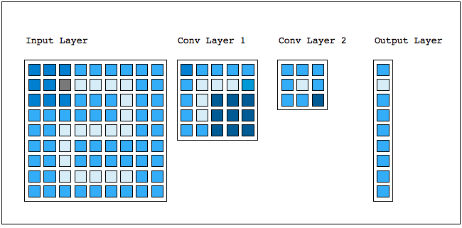
Above example defines the model for a 4-layer network, consisting of 2 hidden convolutional layers in addition to the input and the output layer. The 1st convolutional layer is defined as having 13 x 13 nodes over 5 feature maps, resulting in 845 nodes in total. The 2nd convolutional layer is defined as having 6 x 6 nodes over 5 feature maps, resulting in 180 nodes in total.
I added some code to output the network's characteristics to the console for easier reference.
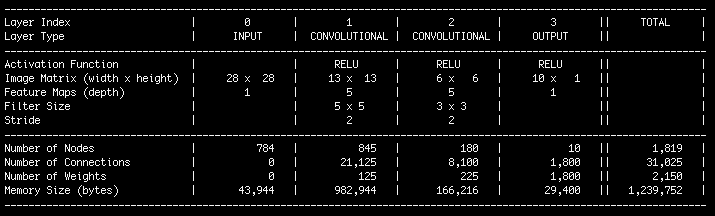
You can see that the network resulting from this model has a total of 2,150 weights and only uses 1.2 MB of memory.
Layer Types
The code currently supports the following types of layers:
1
2typedef enum LayerType {INPUT, CONVOLUTIONAL, FULLY_CONNECTED, OUTPUT} LayerType;
The idea here is that based on the type of layer certain rules are applied, for example, the connections between nodes are created differently.
Moving forward I want to expand this further to include other layer types, for example Hierarchical Temporal Memory (HTM) layers for sequentiell learning.
Activation Function
The code currently supports below 3 activation functions:
1
2typedef enum ActFctType {SIGMOID, TANH, RELU} ActFctType;
Each layer can define its own activation function which is applied during feed forward (activation) as well as during error back propagation. In theory, you can design a network using different activation functions for different layers. In practive, however, this does not improve the network performance.
It's also important to note that other parameters, most significantly the learning rate, depend on what activation function is used. Hence, both of these two hyper-parameters should always be considered in tandem.
Create the Network
Once the network and its layers have been defined via the above setLayerDefinitions function you can create the actual network object via the createNetwork function
1
2Network *nn = createNetwork(numberOfLayers, layerDefs);
which automatically allocates the required memory for this network, initializes its internal structures (see below) and returns a pointer for reference.
 1
 2Network *createNetwork(int layerCount, LayerDefinition *layerDefs){
 3
 4    // Calculate network size
 5    ByteSize netSize = getNetworkSize(layerCount, layerDefs);
 6
 7    // Allocate memory block for the network
 8    Network *nn = (Network*)malloc(netSize);
 9
10    // Set network's default values
11    setNetworkDefaults(nn, layerCount, layerDefs, netSize);
12
13    // Initialize the network's layers, nodes, connections and weights
14    initNetwork(nn, layerCount, layerDefs);
15
16    // Init all weights -- located in the network's weights block after the last layer
17    initNetworkWeights(nn);
18
19    return nn;
20}
Calculate the Network's Memory
To create the network we first need to calculate how much memory it needs. Obviously, this depends on many different parameters, such as the number of layers, the number of nodes per layer, the size of the filter in a convolutional layer, etc.
 1
 2ByteSize getNetworkSize(int layerCount, LayerDefinition *layerDefs){
 3
 4    ByteSize size = sizeof(Network);
 5
 6    for (int i=0; i<layerCount; i++){
 7        ByteSize lsize =getLayerSize(layerDefs+i);
 8        size += lsize;
 9    }
10
11    // get size of weight memory block (located within network, after layers)
12    ByteSize weightBlockSize = getNetworkWeightBlockSize(layerCount, layerDefs);
13
14    // add weight block size to the network
15    size += weightBlockSize;
16
17    return size;
18}
To calculate the network size, we need to calculate each layer's size which in return requires to calculate each column's size which depends on each node's size which depends on the number of connections, ... and so on. You get the idea. Sounds complicated at first, but it's actually pretty straight forward. So, I'm going to skip a review of all the sub functions here. You can review them in the code (see link below).
Initialize the Network
In the above createNetwork function we saw that in addition to setting some default values for the network, we need to initialize the network and set random weights.
Now, what do I mean by initializing the network? Don't forget, until now the network is simply a block of memory with some unknown content inside. We need to insert our desired structure into this memory block so that it mirrors our design as outlined above: a network that holds layers that hold columns that hold nodes that hold connections which point to other nodes and weights. Let's see how this is done.
 1
 2void initNetwork(Network *nn, int layerCount, LayerDefinition *layerDefs){
 3
 4    // Init the network's layers including their backward connections
 5    // Backward connections point to target nodes in the PREVIOUS layer and are used during FEED FORWARD
 6    // (i.e. during calculating node outputs = node activation)
 7    for (int l=0; l<layerCount; l++) initNetworkLayer(nn, l, layerDefs);
 8
 9    // Init the network's forward connections
10    // Forward connections point to target nodes in the FOLLOWING layer that point back to this node, and
11    // and are used during BACK PROPAGATION (to speed-up calculating the proportional error)
12    for (int l=0; l<layerCount; l++) initNetworkForwardConnections(nn, l);
13
14}
First, we loop through all layers and initialize them one by one. After that, we loop again to set up each layer's forward connections.
The reason why we need 2 loops here is that in order for the initNetworkForwardConnections function to work, each layer's following layer must have been initialized already.
The background is simple: initNetworkForwardConnections checks which nodes in the following layer point back to a node in this layer and then creates forward connections mirroring these backward connections.
Obviously, if the following layer hadn't been setup yet, there wouldn't be any forward connections in this layer. Hence, 2 loops.
Now, let's see what actually happens inside the initNetworkLayer function:
 1
 2void initNetworkLayer(Network *nn, int layerId, LayerDefinition *layerDefs){
 3
 4    LayerDefinition *layerDef = layerDefs + layerId;
 5
 6    // Calculate the layer's position by moving a single byte pointer forward
 7    // by the total sizes of all previous layers
 8    uint8_t *sbptr1 = (uint8_t*) nn->layers;
 9    for (int l=0; l<layerId; l++) sbptr1 += getLayerSize(layerDefs+l);
10    Layer *layer = (Layer*) sbptr1;
11
12    // Calculate the position of this layer's weights block
13    uint8_t *sbptr2 = (uint8_t*) nn->weightsPtr;
14    for (int l=0; l<layerId; l++) sbptr2 += getLayerWeightBlockSize(layerDefs+l);
15    Weight *w = (Weight*) sbptr2;
16
17    // Set default values for this layer
18    layer->id              = layerId;
19    layer->layerDef        = layerDef;
20    layer->weightsPtr      = w;
21    layer->size            = getLayerSize(layerDef);
22    layer->columnCount     = getColumnCount(layerDef);
23
24    // Initialize all columns inside this layer
25    initNetworkColumns(nn, layerId);
26
27}
In order to initialize a layer, we first need to know where each layer starts.
Remember, since each layer has a different size, I cannot use a simple array reference such as network.layer[1] to locate a layer.
Instead, I point a single byte pointer to the start of the network's layers nn->layers and move it forward by exactly the size of each layer.
Then, I define for each layer some basics such as its id, its weightPtr, etc., and add a reference to its original LayerDefinition.
This will become handy because througout the code we will need to access a layer's definition quite often.
Now, we've setup the head of the layer. What's missing is the structure underneath, i.e. the columns inside this layer. So that's what's next.
 1
 2void initNetworkColumns(Network *nn, int layerId){
 3
 4    Layer *layer = getNetworkLayer(nn, layerId);
 5
 6    int backwardConnCount = getNodeBackwardConnectionCount(layer->layerDef);
 7    int forwardConnCount  = getNodeForwardConnectionCount(layer->layerDef);
 8
 9    ByteSize columnSize = getColumnSize(layer->layerDef);
10
11    // Init all columns attached to this layer
12    for (int c=0; c<layer->columnCount; c++){
13
14        // Set pointer to the respective column position (using a single byte pointer)
15        uint8_t *sbptr = (uint8_t*) layer->columns;
16        sbptr += c * columnSize;
17
18        Column *column = (Column*) sbptr;
19
20        // Set default values of a node
21        column->size     = columnSize;
22        column->nodeCount= layer->layerDef->nodeMap.depth;
23        column->maxConnCountPerNode = backwardConnCount+forwardConnCount;
24
25        // Initialize all nodes of a column
26        initNetworkNodes(nn, layerId, c);
27
28    }
29
30}
Again, the same logic as above applies. Since the size of a column structure is variable I use a single byte pointer to determine the starting point of each column inside this layer. Once I've done that, I continue to intitialize all of the nodes inside this column.
 1
 2void initNetworkNodes(Network *nn, int layerId, int columnId){
 3
 4    Layer *thisLayer    = getNetworkLayer(nn, layerId);
 5    Layer *prevLayer    = getNetworkLayer(nn, layerId-1);
 6    Column *column      = getLayerColumn(thisLayer, columnId);
 7    ByteSize nodeSize   = getNodeSize(thisLayer->layerDef);
 8
 9    uint8_t *sbptr = (uint8_t*) column->nodes;
10
11    // Create a vector containing the ids of the target columns (conv layers only)
12    Vector *filterColIds = createFilterColumnIds(thisLayer, columnId, prevLayer);
13
14    // Init all nodes attached to this column
15    for (int n=0; n<column->nodeCount; n++){
16
17        // Set pointer to the respective node position (using a single byte pointer)
18        Node *node = (Node*) sbptr;
19        sbptr += nodeSize;
20
21        // Reset node's defaults
22        setNetworkNodeDefaults(thisLayer, column, node, &nn->nullWeight);
23
24        // Initialize backward connections of fully-connected layer node
25        if (thisLayer->layerDef->layerType==FULLY_CONNECTED || thisLayer->layerDef->layerType==OUTPUT){
26
27            int nodeId = (columnId * column->nodeCount) + n;
28
29            // @attention When calculating the weightsId, only consider backwardConnections
30            int layerWeightsId = nodeId * getNodeBackwardConnectionCount(thisLayer->layerDef);
31            Weight *nodeWeight = thisLayer->weightsPtr + layerWeightsId;
32
33            initNetworkBackwardConnectionsFCNode(node, prevLayer, nodeWeight);
34        }
35
36        // Initialize backward conections of convolutional layer node
37        if (thisLayer->layerDef->layerType==CONVOLUTIONAL){
38            // @attention Nodes on the same level share the same weight block
39            initNetworkBackwardConnectionsConvNode(node, n, thisLayer->weightsPtr, prevLayer, filterColIds, &nn->nullWeight);
40        }
41
42    }
43
44    free(filterColIds);
45}
Create Backward Connections
This function is central to the network's initialization process.
In addition to setting some default values for all nodes, it's preparing the creation of backward connections of each node to the previous layer.
The way in which these backward connections are constructed is obviously different for fully connected and for convolutional layers.
Hence there are 2 different sub functions, initNetworkBackwardConnectionsFCNode for fully connected nodes and initNetworkBackwardConnectionsConvNode for convolutional nodes.
Backward Connections for Fully Connected Layers
Let's look at the easier of the 2 first, the fully connected node:
 1
 2void initNetworkBackwardConnectionsFCNode(Node *thisNode, Layer *prevLayer, Weight *nodeWeightPtr){
 3
 4    int connId = 0;
 5    int nodeWeightId = 0;
 6
 7    ByteSize columnSize = getColumnSize(prevLayer->layerDef);
 8
 9    uint8_t *sbptr_column = (uint8_t*) prevLayer->columns;
10
11    for (int col=0; col<prevLayer->columnCount;col++){
12
13        Column *column = (Column *)sbptr_column;
14
15        uint8_t *sbptr_node = (uint8_t*) column->nodes;
16
17        for (int n=0; n<column->nodeCount; n++){
18
19            Connection *conn = &thisNode->connections[connId];
20
21            conn->weightPtr = nodeWeightPtr + nodeWeightId;
22
23            conn->nodePtr = (Node *)sbptr_node;
24
25            sbptr_node += getNodeSize(prevLayer->layerDef);
26
27            connId++;
28            nodeWeightId++;
29        }
30        sbptr_column += columnSize;
31    }
32}
The function loops through the previous layer's nodes and creates a connection from the current node to each node in the previous layer (hence fully connected). Remember, since nodes are structured in columns we need to loop through the columns first and then through the nodes inside each column.
So far so good. That was the easier of the two. Now, let's look at how the wiring (building connections) works for convolutional nodes.
Backward Connections for Convolutional Layers
As outlined above, a convolutional node is connected to a selected group of neighboring nodes, located within a quadratic region of filter size.
This quadratic region (the filter) needs to be calculated.
It depends on a number of parameters and changes as the filter is moved across the target layer.
Example: Let's say our network consists of 3 layers, the input layer containing the MNIST image, a convolutional layer and the output layer.
We know that the MNIST image has 28*28 pixels, hence the input layer has 784 columns. Each column only has 1 node (the depth of the input layer is 1) therefore there are also exactly 728 nodes. And let's assume our convolutional layer has dimensions of [24 * 24 * 10], i.e. there are 24 * 24 = 576 columns and each column has 10 nodes. And let's assume we defined a filter of 5 for this layer.
Now we start wiring up the 1st node in the convolutional layer. We need to create connections to a region of 5 x 5 (filter * filter size) columns located at the top left of the target (in this case = input) layer. The respective ids of these columns would be:
1[   0,   1,   2,   3,   4,
2   28,  29,  30,  31,  32,
3   56,  57,  58,  59,  60,
4   84,  85,  86,  87,  88,
5  112, 113, 114, 115, 116]
Then we move on to the 2nd node in the convolutional layer. Again, we create connections to a 5 x 5 region, but the region now moved to right along with the convolutional (source) node itself. Hence, the target column ids of the 2nd node in the convolutional layer would be:
1[   1,   2,   3,   4,   5,
2   29,  30,  31,  32,  33,
3   57,  58,  59,  60,  61,
4   85,  86,  87,  88,  89,
5  113, 114, 115, 116, 117]
Above calculation is done by the calcFilterColumnIds function below.
I trust you'll be able to walk through it, using the logic introduce in the example above.
 1
 2void calcFilterColumnIds(Layer *srcLayer, int srcColId, Layer *tgtLayer, Vector *filterColIds){
 3
 4    int srcWidth  = srcLayer->layerDef->nodeMap.width;
 5    int tgtWidth  = tgtLayer->layerDef->nodeMap.width;
 6    int tgtHeight = tgtLayer->layerDef->nodeMap.height;
 7
 8    int filter = srcLayer->layerDef->filter;
 9    int stride = calcStride(tgtWidth, filter, srcWidth);
10
11    int startX = (srcColId % srcWidth) * stride;
12    int startY = floor((double)srcColId/srcWidth) * stride;
13    int id=0;
14
15    for (int y=0; y<filter; y++){
16
17        for (int x=0; x<filter; x++){
18
19            int colId = ( (startY+y) * tgtWidth) + (startX+x);
20
21            // Check whether target columnId is still within the target node range
22            // If NOT then assign a dummy ID ("OUT_OF_RANGE") that is later checked for
23            if (
24                (floor(colId / tgtWidth) > (startY+y)) ||  // filter exceeds nodeMap on the right
25                (colId >= tgtWidth * tgtHeight)            // filter exceeds nodeMap on the bottom
26                ) colId = OUT_OF_RANGE;
27
28            filterColIds->vals[id] = colId;
29            id++;
30        }
31    }
32}
Once we calculated this vector of targetColumnIds we pass it into our initNetworkBackwardConnectionsConvNode function which then creates connections from the source node to the target nodes specified in the vector.
 1void initNetworkBackwardConnectionsConvNode(Node *node, int srcLevel, Weight *srcLayerWeightPtr, Layer *targetLayer, Vector *filterColIds, Weight *nullWeight){
 2
 3    int filterSize = filterColIds->count;
 4    int tgtDepth   = targetLayer->layerDef->nodeMap.depth;
 5
 6    for (int posInsideFilter=0; posInsideFilter<filterSize; posInsideFilter++){
 7
 8        int targetColId = (int)filterColIds->vals[posInsideFilter];
 9
10        for (int tgtLevel=0; tgtLevel<tgtDepth; tgtLevel++){
11
12            Connection *conn = &node->connections[ (tgtLevel*filterSize)+posInsideFilter];
13
14            if (targetColId!=OUT_OF_RANGE){
15
16                int weightPosition = (srcLevel*(tgtDepth*filterSize)) + (tgtLevel*filterSize) + posInsideFilter;
17
18                Weight *tgtWeight = srcLayerWeightPtr + weightPosition;
19
20                Node *tgtNode = getNetworkNode(targetLayer, targetColId, tgtLevel);
21
22                conn->nodePtr   = tgtNode;
23                conn->weightPtr = tgtWeight;
24            }
25            else {
26            // if filter pixel is out of range of the target nodes then point to NODES if THIS layer
27            // this kind of pointer needs to be captured later i.e. should NOT be CALCULATED/ACTIVATED
28            conn->nodePtr   = NULL;
29            conn->weightPtr = nullWeight;
30            }
31        }
32    }
33}
Depending on how many nodes we defined in our convolutional layer, some of the nodes in the target (=previous) layer are purposely skipped.
This is called the stride. A stride of 2 means that every other node in the target layer is skipped.
The idea is to downsize the original image layer by layer, and have each following layer represent some higher level feature of the previous layer.
1int calcStride(int tgtWidth, int filter, int srcWidth){
2  return ceil(((double)tgtWidth - filter)/(srcWidth-1));
3}
Create Forward Connections
What are forward connections and why do we need them? Let's revisit some of the above. A connection links 2 nodes and applies a weight during the feed forward process. Then, during the back propagation process, the same connection is traversed in opposite direction to pass the partial error of a node back to the connected node in the previous layer. It's the latter that triggered the need for forward connections.
How? C pointers are one-directional. Variable A points to variable B but variable B does not know who points to it. Therefore, I cannot simply traverse a connection between nodes in opposite direction. So instead, I create additional connections from the target back to the source.
Both types of connections, backward and forward, serve different purposes:
1Backward connections are used during feed forward.
1Forward connections are used during back propagation.
Yes, that's no typo. The above may sound counter-intuitive at first, but makes sense when you think about it.
During feed forward you need to calculate the output of a node. To do so, you need to loop through all of its incoming (=backward) nodes to calculate the vector product and apply an activation function to the output.
During back propagation you need to calculate the error of a node. To do so, you need to loop through all its outgoing (=forward) nodes to obtain the partial error from this node and apply a derivative function.
So, here's the function for initializing the network's forward connection:
 1void initNetworkForwardConnections(Network *nn, int layerId) {
 2
 3    // Skip the first=INPUT and the last=OUTPUT layer because they don't have forward connections
 4    if (layerId==0 || layerId==nn->layerCount-1) return;
 5
 6    Layer *thisLayer = getNetworkLayer(nn, layerId);
 7    Layer *nextLayer = getNetworkLayer(nn, layerId+1);
 8
 9    for (int c=0; c<thisLayer->columnCount; c++){
10
11        Column *column = getLayerColumn(thisLayer, c);
12
13        for (int n=0; n<column->nodeCount; n++){
14            Node *node = getColumnNode(column, n);
15            initNetworkForwardConnectionsAnyNode(node, nextLayer);
16        }
17    }
18}
It simply loops through all layers and their respective columns and calls the initNetworkForwardConnectionsAnyNode function which does the actual wiring:
 1void initNetworkForwardConnectionsAnyNode(Node *thisNode, Layer *nextLayer) {
 2
 3    int maxForwardConnCount = thisNode->forwardConnCount;
 4    int forwardConnStart = thisNode->backwardConnCount;
 5    int forwardConnCount = 0;
 6
 7    for (int o=0;o<nextLayer->columnCount;o++){
 8        for (int n=0; n<nextLayer->columns[0].nodeCount; n++){
 9
10            Node *nextLayerNode = getNetworkNode(nextLayer,o, n);
11            for (int c=0;c<nextLayerNode->backwardConnCount;c++){
12
13                // If the connection of the node in the next layer points back to this node
14                // then store this nextNode as a target in the forwardConnections of this node
15                // and point the connection to the same weight
16                if (nextLayerNode->connections[c].nodePtr == thisNode) {
17                    thisNode->connections[forwardConnStart + forwardConnCount].nodePtr = nextLayerNode;
18                    thisNode->connections[forwardConnStart + forwardConnCount].weightPtr = nextLayerNode->connections[c].weightPtr;
19                    forwardConnCount++;
20                    if (forwardConnCount>maxForwardConnCount) {
21                        printf("Maximum forward connections exceeded! ABORT!\n\n");
22                        exit(1);
23                    }
24                }
25            }
26        }
27    }
28    thisNode->forwardConnCount = forwardConnCount;
29}
Initialize Weights
Now that we've fully setup all of the connections between the nodes and from the nodes to their weights, we still need to initialize the weights.
Remember, all weights are located in a big weight block at the end of the Network structure.
All we need to do is initialize each weight with a random value from 0-1. For better performance I found that it helps to reduce the value to a random number smaller than 0.5 or 0.4 and also to make every other weight negative.
 1void initNetworkWeights(Network *nn){
 2
 3    // Init weights in the weight block
 4    for (int i=0; i<nn->weightCount; i++){
 5        Weight *w = &nn->weightsPtr[i];
 6        *w = 0.4 * (Weight)rand() / RAND_MAX;   // multiplying by a number <0 results in better performance
 7        if (i%2) *w = -*w;                      // make half of the weights negative (for better performance)
 8    }
 9
10    // Init weights in the nodes' bias
11    for (int l=0; l<nn->layerCount;l++){
12        Layer *layer = getNetworkLayer(nn, l);
13        for (int c=0; c<layer->columnCount; c++){
14            Column *column = getLayerColumn(layer, c);
15            for (int n=0; n<column->nodeCount; n++){
16                // init bias weight
17                Node *node = getColumnNode(column, n);
18                node->bias = (Weight)rand()/(RAND_MAX);
19                if (n%2) node->bias = -node->bias;  // make half of the bias weights negative
20            }
21        }
22    }
23}
Train the Network
Once the network has been fully setup and initialized, we can train it in exactly the same manner as described in my previous post:
1
21. read an image
32. feed it into the input layer of the network
43. feed all layers forward applying an activation function each time
54. backpropagate the error through all layers and update its weights
To obtain some indication of the network's progress during the training process we can count the number of correct classifications versus the total number of images and calculate an ongoing accuracy rate.
 1void trainNetwork(Network *nn){
 2
 3    // open MNIST files
 4    FILE *imageFile, *labelFile;
 5    imageFile = openMNISTImageFile(MNIST_TRAINING_SET_IMAGE_FILE_NAME);
 6    labelFile = openMNISTLabelFile(MNIST_TRAINING_SET_LABEL_FILE_NAME);
 7
 8    int errCount = 0;
 9
10    // Loop through all images in the file
11    for (int imgCount=0; imgCount<MNIST_MAX_TRAINING_IMAGES; imgCount++){
12
13        // Reading next image and its corresponding label
14        MNIST_Image img = getImage(imageFile);
15        MNIST_Label lbl = getLabel(labelFile);
16
17        // Convert the MNIST image to a standardized vector format and feed into the network
18        Vector *inpVector = getVectorFromImage(&img);
19        feedInput(nn, inpVector);
20
21        // Feed forward all layers (from input to hidden to output) calculating all nodes' output
22        feedForwardNetwork(nn);
23
24        // Back propagate the error and adjust weights in all layers accordingly
25        backPropagateNetwork(nn, lbl);
26
27        // Classify image by choosing output cell with highest output
28        int classification = getNetworkClassification(nn);
29        if (classification!=lbl) errCount++;
30    }
31    // Close files
32    fclose(imageFile);
33    fclose(labelFile);
34}
Once the network has been trained on the the 50,000 images in the training set (no distinction between training and validation set is made), we stop training and run the network on the 10,000 images in the testing set.
Test the Network
The process during testing is exactly the same as during training, the only difference is that we switch off the learning, i.e. we don't back propagate the error and don't update any weights.
 1void testNetwork(Network *nn){
 2
 3    // open MNIST files
 4    FILE *imageFile, *labelFile;
 5    imageFile = openMNISTImageFile(MNIST_TESTING_SET_IMAGE_FILE_NAME);
 6    labelFile = openMNISTLabelFile(MNIST_TESTING_SET_LABEL_FILE_NAME);
 7
 8    int errCount = 0;
 9
10    // Loop through all images in the file
11    for (int imgCount=0; imgCount<MNIST_MAX_TESTING_IMAGES; imgCount++){
12
13        // Reading next image and its corresponding label
14        MNIST_Image img = getImage(imageFile);
15        MNIST_Label lbl = getLabel(labelFile);
16
17        // Convert the MNIST image to a standardized vector format and feed into the network
18        Vector *inpVector = getVectorFromImage(&img);
19        feedInput(nn, inpVector);
20
21        // Feed forward all layers (from input to hidden to output) calculating all nodes' output
22        feedForwardNetwork(nn);
23
24        // Classify image by choosing output cell with highest output
25        int classification = getNetworkClassification(nn);
26        if (classification!=lbl) errCount++;
27    }
28    // Close files
29    fclose(imageFile);
30    fclose(labelFile);
31}
Output Classification
In case you wondered how the classification of an image in the output layer is done: I'm not using a softmax or similar function. Instead, I'm simply comparing all outputs of the 10 nodes in the output layer with each other and take the highest. :-)
 1int getNetworkClassification(Network *nn){
 2
 3    Layer *l = getNetworkLayer(nn, nn->layerCount-1);   // get output layer
 4
 5    Weight maxOut = 0;
 6    int maxInd = 0;
 7
 8    for (int i=0; i<l->columnCount; i++){
 9        Node *on = getNetworkNode(l,i,0); // the output layer always has a depth of 1
10        if (on->output > maxOut) {
11            maxOut = on->output;
12            maxInd = i;
13        }
14    }
15    return maxInd;
16}
That's it. Now that we've done all the coding, let's look at performance.
Network Performance
To assess the performance of the network let's look at its accuracy as well as its speed. Here's a summary of the different network designs that I tried and their respective best results:
 1TEST RESULTS
 2
 3| Network     | # of Nodes     | Act.Fct | L-Rate | # Trains | Speed* | Accuracy || Compare** |
 4| ----------- |----------------|---------|--------|----------|--------|----------||-----------|
 5| 1-l   FC NN |      10 output | SIGMOID | 0.0125 |  900,000 |   228s |   91.09% ||    88.00% |
 6| 2-l   FC NN |     300 hidden | SIGMOID | 0.0700 |  120,000 |   697s |   94.67% ||    96.40% |
 7| 3-l   FC NN | 500+150 hidden | SIGMOID | 0.0050 |  180,000 | 2,510s |   93.64% ||    97.05% |
 8| 3-l ConvNet | 13x13x5, 6x6x5 |  RELU   | 0.0004 |  525,000 |   908s |   88.40% ||    98.90% |
 9
10 * total run-time in seconds, including training and testing, on a 2010 MacBook Pro
11** best accuracies listed on http://yann.lecun.com/exdb/mnist/ (without pre-processing)
As you can see from the above my network is doing well for smaller models but not so much for larger, deeper structures. This is not due to wrong coding. It's because I haven't used the most efficient parameters during the training.
This leads us to the most difficult part of machine learning: How to find the hyper-parameters that achieve the best results?
Hyper-parameter Optimization
Surprisingly, optimizing hyper-parameters such as the learning rate or the number of nodes is still mostly a manual process. Based on my reading it seems that techniques such as grid search or Bayesian Optimization work equally good or bad than a Random Search does.
Therefore, I plan to dedicate my next post to the topic of network parameter fine tuning and build my own optimization tool to get some bettter results from my network. Stay tuned! :)
Code & Documentation
As always you can find all the code for this exercise on my Github project page, including full code documentation.
Happy Hacking!
![]()